Science
Princeton's T16 search finds 10,091 new TESS planet candidates around faint stars
A GPU transit search and two random forests combed 83.7 million TESS light curves, down to 16th-magnitude stars, and turned up 11,554 planet candidates.
HackHoster Team · · 11 min read
At a glance
- Princeton's T16 team searched 83.7 million light curves from TESS's first year and reports 11,554 planet candidates; 10,091 are new signals with multiple transits.
- The search reaches stars down to TESS magnitude 16, roughly ten times fainter than the 13.5 cutoff used by most earlier systematic searches.
- Two scikit-learn random forests, one built for faint stars, scored each signal on 53 features; the paper reports a weighted F1 score of 0.91.
- About 50,000 signals were inspected by eye, and the authors warn the list may still hold more eclipsing binaries than a typical catalog.
- Magellan radial velocities confirmed TIC 183374187 b, a hot Jupiter on a 5.06-day orbit around a metal-poor star about 12 billion years old.
- The catalog, vetting plots, and light curves are public, and the authors say the search used only about 15% of the TESS data available.
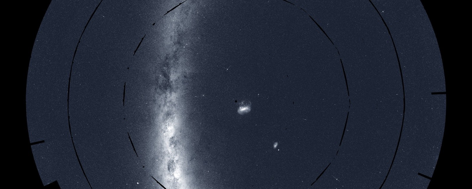
A team led by Joshua T. Roth at Princeton University published the T16 Planet Hunt in The Astrophysical Journal Supplement Series on April 28, eight days after posting the preprint. They searched every light curve their group had built from the first year of NASA's Transiting Exoplanet Survey Satellite (TESS), 83,717,159 of them, and report 11,554 planet candidates with orbital periods between half a day and 27 days.
Of those, 10,091 are new candidates with at least two transits, so their orbits can be measured. Another 411 are new single-transit events, and 1,052 were already known. The paper says the haul multiplies the number of candidates found in TESS data by about 2.4, using only the mission's first observing cycle.
The difference from earlier searches is depth. Most systematic TESS planet searches stopped at stars brighter than magnitude 13.5 in the TESS band. T16 goes down to magnitude 16, which is where the project gets its name, and about 70% of the candidates orbit stars fainter than the old cutoff.
Why faint stars were left out
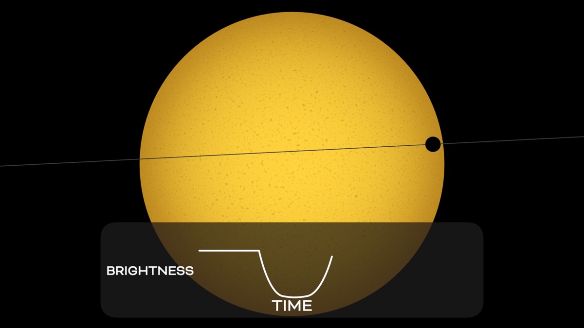
The transit method has been astronomy's most productive way to find planets since HD 209458 b was caught crossing its star in 1999. The paper puts its share at about three quarters of all confirmed exoplanets. A planet that passes in front of its star blocks a small fraction of the starlight once per orbit, and a telescope that watches the star's brightness long enough sees a repeating dip.
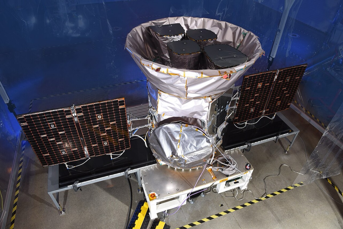
TESS was built to do that across almost the whole sky. It launched on April 18, 2018, according to NASA, and it is now in its third extended mission. As of March 12, 2026, the paper counts nearly 8,000 TESS planet candidates, of which 760 had been confirmed.
Those numbers lean heavily toward bright stars, and the reason is practical. A candidate only becomes a planet after follow-up, usually radial-velocity measurements that detect the star wobbling under the planet's pull, and faint stars need much more telescope time for that. Pipelines built to feed follow-up programs set magnitude limits to match.
Yield studies, though, predicted tens of thousands of detectable planets around fainter TESS targets. The authors explain why: transit surveys are limited by signal-to-noise, not by brightness as such. A large planet such as a hot Jupiter blocks enough light to stay detectable around distant stars, so the volume of space you can search grows quickly as you go fainter. Stopping at magnitude 13.5 leaves most of that volume unexamined.
What "T16" means. Astronomical magnitudes run backwards and on a log scale: a difference of 5 magnitudes is a factor of 100 in brightness. The TESS-band limit of 16 is 2.5 magnitudes fainter than the common 13.5 cutoff, so the faintest T16 stars are about ten times dimmer than the faintest stars in earlier searches. It is a magnitude limit, not a "16 times fainter" factor, as some coverage put it.
From full-frame images to light curves
TESS has four wide-field cameras, each with a 10 cm aperture, imaging onto four CCDs of 2048 by 2048 pixels. Its first year was split into 13 sectors, each observed for two spacecraft orbits of 13.7 days, giving each light curve a baseline of about 27 days. Each pixel spans roughly 21 arcseconds of sky, which matters later: light from several stars can land in the same pixel.
Besides preselected targets, TESS saves full-frame images. In the first year, its 2-second exposures were summed into a full-frame image every 30 minutes. Those images contain tens of millions of stars nobody selected in advance.
The T16 light curves come from a 2025 paper by Joel Hartman, Gáspár Bakos, Luke Bouma, and Zoltan Csubry; the first three are also co-authors of the new search. Instead of measuring each star directly, they used difference imaging:
- Build a sharp reference frame by aligning and stacking about 50 science frames.
- Subtract the reference from every frame, so constant stars and background vanish and only changes in brightness remain.
- Place apertures at each star's position from the Gaia catalog, and take each star's baseline brightness from Gaia rather than from the blurry TESS image, which helps in crowded fields.
- Remove spacecraft systematics with two detrending passes run in VARTOOLS: a spline-based decorrelation against time, CCD position, and temperature, then the Trend Filtering Algorithm, which fits each light curve against 200 quiet template stars on the same detector.
The result is 83,717,159 light curves, more than one per star because many stars fall in several sectors. The two papers give slightly different star counts: the 2025 light-curve paper says 56,401,549, and the planet-hunt paper says 54,401,549. Either way it is tens of millions of stars, and the light curves are public through NASA's MAST archive as the high-level science product "t16".

A GPU search, then two random forests
Searching 80 million light curves for periodic dips is expensive, so the first step uses CETRA, the Cambridge Exoplanet Transit Recovery Algorithm. CETRA scans each light curve for single transit-shaped dips, then folds those detections over a grid of trial periods. Its 2025 paper reports that it finds at least 20% more low signal-to-noise transits than Transit Least Squares in the same data, runs up to a few orders of magnitude faster on high-cadence light curves, and is open source on GitHub and PyPI, built on NVIDIA's CUDA. The T16 authors say speed was CETRA's main advantage for them.
CETRA returns a period but not much else, so the team re-ran the classic Box Least Squares (BLS) statistic at that period and at half, double, and triple it. Comparing those harmonics is a standard way to tell a planet from an eclipsing binary, whose two eclipses per orbit can fool a search into finding half the true period. That produced 87 parameters per light curve. After dropping ones that shouldn't matter, such as raw brightness, and adding each star's temperature and luminosity from Gaia, 53 features remained.
Why random forests
The authors chose random forest classifiers over deep networks on raw light curves, for three reasons they spell out: forests are cheap enough to run on millions of inputs, they report which features drive each decision, and they cope with noisy or missing values. They used scikit-learn's implementation.
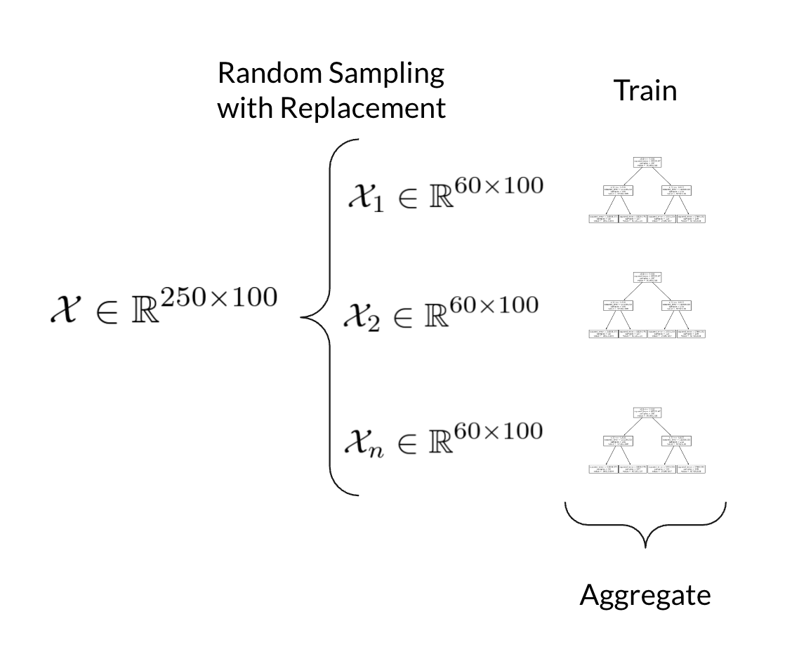
A single forest didn't work well across the whole brightness range, because faint stars are much noisier. So there are two: a base model, and a faint-star model for stars at magnitude 14.5 and fainter. Both sort signals into three classes: no signal, eclipsing binary, or planetary transit.
The hard part was training data for faint stars, where almost no confirmed examples exist. The team made up the gap by injecting synthetic eclipses and transits into real light curves, keeping an injection only if CETRA recovered its period to within 1%.
| Training examples | Base model | Faint-star model |
|---|---|---|
| Light curves with no signal | 9,342 | 5,940 |
| Real eclipsing binaries recovered | 6,395 | 1,160 |
| Injected eclipsing binaries | 2,309 | 7,298 |
| Real TESS Objects of Interest recovered | 3,632 (from 2,095 TOIs) | 91 |
| Injected planetary transits | 1,456 | 8,517 |
Training ran twice per model: once on all features with a grid search, then again on the 30 most important ones to curb overfitting. On a 20% hold-out set, the paper reports a weighted F1 score of 0.91 and ROC AUC of 0.99 for the no-signal class and 0.98 for transits and binaries. The base model labeled 87% of held-out transits correctly; the faint model, 93%. The single most useful feature for both was the signal-to-pink-noise ratio of the strongest CETRA peak, a measure that accounts for correlated noise.
To pick a probability cutoff, the team vetted about 1,500 light curves by hand and compared their calls with the model's. They settled on 0.5, meaning a signal is kept if the forest thinks it is more likely a transit than not.
The vetting funnel
A classifier score is the start of vetting, not the end. The biggest enemy is the eclipsing binary: two stars orbiting each other produce dips that look like transits, and with 21-arcsecond pixels, a binary next to a target can leak its eclipses into the target's light curve.
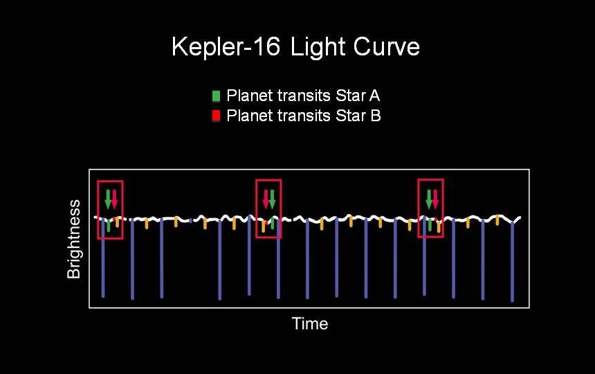
The automated steps, in order:
- Contamination groups. Using the NetworkX library, the pipeline links every pair of flagged stars within two arcminutes that share a compatible period and timing. In each linked group, only the star with the strongest signal survives; the rest are treated as blends.
- Signal strength. Candidates need a signal-to-pink-noise ratio above 10.
- Systematics. If too many signals on one CCD share a period and transit times, they are removed as instrument artifacts.
- Size. A quick transit-model fit throws out anything whose implied planet radius exceeds 2.5 times Jupiter's.
- Centroids. For each candidate, a 25-by-25-pixel cutout compares the image in and out of transit. If the dimming sits off the target star, the candidate is dropped.
- A second forest. Trained on about 4,500 hand-labeled candidates and tuned for recall, it removes about half the remaining false positives while keeping 98% of signals humans judged real.
That left about 50,000 candidates, every one of which was inspected by at least one person using a standard set of vetting plots. After matching against known eclipsing-binary catalogs, 13,880 signals from 11,554 distinct stars remained.
Read the caveat before you point a telescope. The authors say that with this many candidates, a very thorough look at each one wasn't feasible, so the list may contain more eclipsing binaries and other false positives than usual. They recommend checking the published vetting plot for any candidate before spending follow-up time on it.
What the catalog contains
| Measure | Value |
|---|---|
| Light curves searched | 83,717,159 |
| Candidates after automated steps | about 50,000 (all inspected by eye) |
| Final candidates | 11,554 |
| New, with two or more transits | 10,091 |
| New, single transit | 411 |
| Previously known TESS candidates | 1,052 |
| Gas-giant-size candidates | 97.7% |
| Ultra-short-period candidates (under 1 day) | 66 |
| Possible super-Earths | 11 |
| Hosts that are K / G / F / M stars | 37.3% / 33.5% / 18.2% / 5.2% |
The period distribution peaks around 3.5 days, matching the well-known pile-up of hot Jupiters between 3 and 5 days. The authors stress that this does not represent the true population: transits get rarer at longer periods, and a single 27-day sector makes periods beyond about 13 days hard to catch.
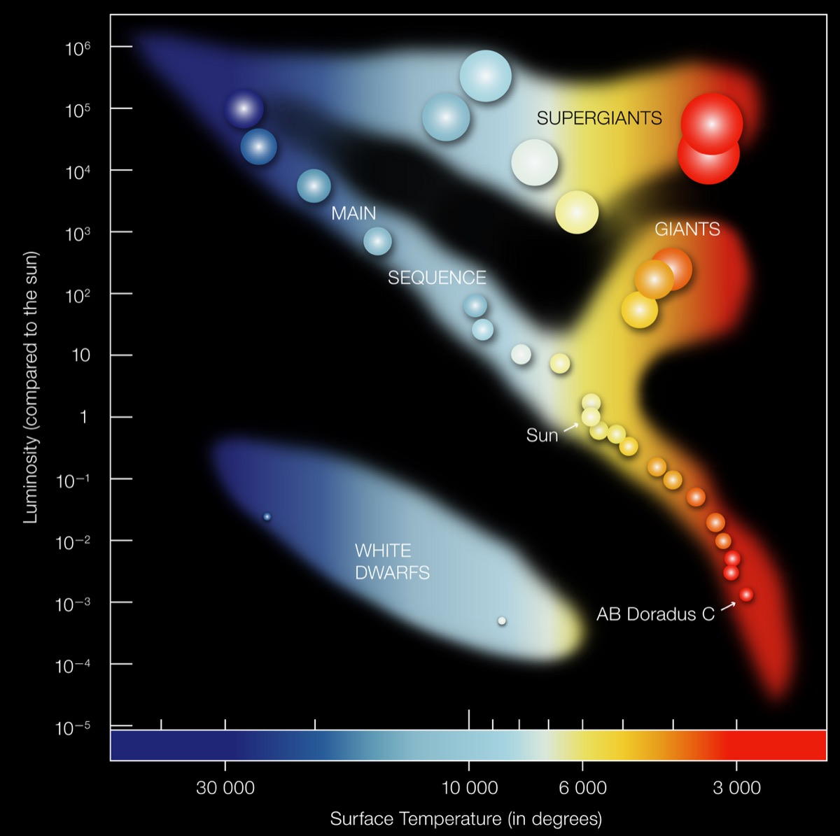
Some subsets stand out for science. The catalog has 737 candidates around low-metallicity stars, which could belong to the Milky Way's old thick disk or even its halo, and a large number of candidates around late M dwarfs, which the authors see as a way to study how short-period giant planets form and survive around small stars. Of the 3,338 candidates brighter than magnitude 13.5, most had already been flagged as threshold-crossing events by the official pipelines, yet 2,479 were never promoted to TESS Objects of Interest.
One planet confirmed so far
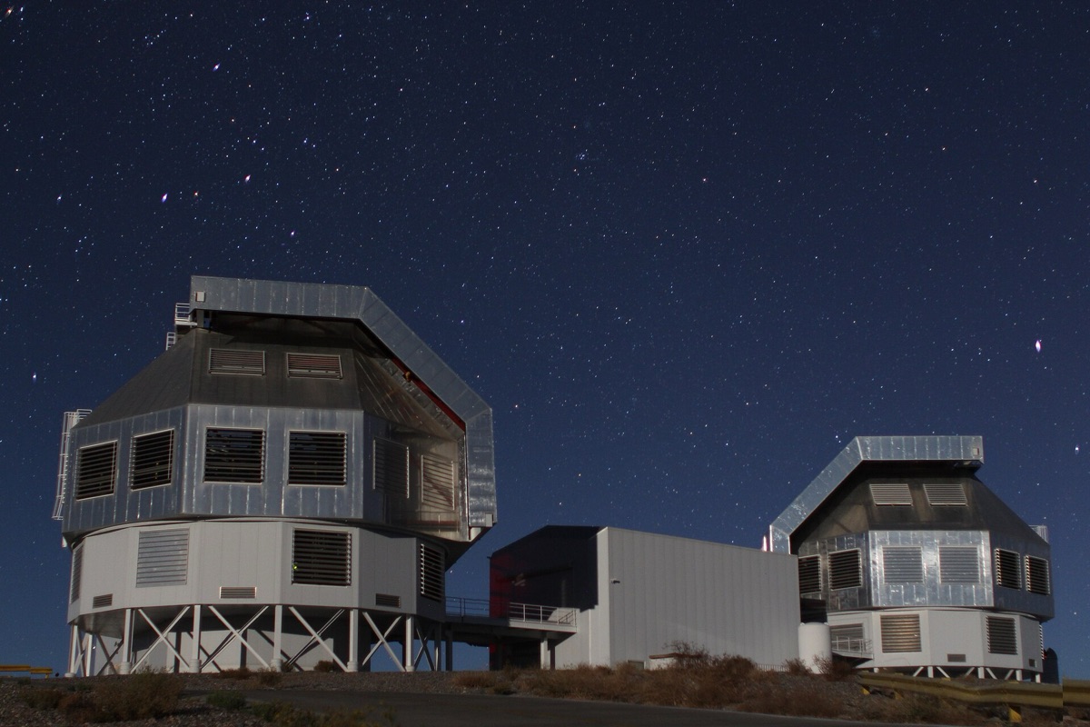
To show the pipeline finds real planets, the team followed up one candidate with the Planet Finder Spectrograph on the 6.5-meter Magellan Clay telescope at Las Campanas Observatory in Chile. Seven radial-velocity measurements over two observing runs confirmed TIC 183374187 b.
| TIC 183374187 | Value |
|---|---|
| Orbital period | 5.059 days |
| Planet mass | about 0.56 to 0.58 Jupiter masses |
| Planet radius | 1.25 Jupiter radii |
| Host temperature | 5,768 K |
| Host metallicity [Fe/H] | −0.39 |
| Host age | about 12.3 billion years |
| Distance | about 1,218 parsecs |
The host is interesting on its own. Its motion through the galaxy places it in the thick disk, and the team measured its chemistry with the spectrograph's high-resolution mode, finding the enhanced magnesium and other alpha elements typical of that old population. A blend analysis strongly favored a planet over a hierarchical triple star system or a background eclipsing binary. The fit hints at a slightly eccentric orbit, but the authors show it is consistent with a circular one.
Limits and open questions
The confirmation shows the pipeline can find real planets, but the paper is careful to say it doesn't measure the false-positive rate or the detection completeness. Those need injection-recovery tests across all the light curves, which the authors estimate would cost more compute than the six-month search itself, though GPU servers roughly 50 times faster than their hardware could make it feasible.
Completeness is visibly imperfect. Of 1,629 known first-year TESS Objects of Interest that the pipeline could in principle recover, it missed 766. The forest had accepted 709 of those; manual vetting removed 72, and the conservative contamination, systematics, and radius filters removed the rest. The authors accept that trade to keep confidence in the new candidates, and suggest looser cuts in future work.
Follow-up is the other bottleneck. The paper estimates that one useful radial-velocity point for a Jupiter-mass planet on a 10-day orbit around a magnitude-16 Sun-like star takes about 0.8 hours with the Magellan spectrograph, while a 10-Earth-mass super-Earth around the same star would need about 820 hours. Ruling out eclipsing binaries is far cheaper, since two low-precision velocities can do it.
Coverage should also be read carefully. Some reports described the search as covering 83.7 million stars; the papers say 83.7 million light curves from roughly 54 to 56 million stars.
What builders can do with it
Everything needed to work with this catalog is public:
- The catalog. Machine-readable tables are published with the journal paper, and the candidates are being submitted as community TESS Objects of Interest.
- The vetting plots. One summary plot per candidate is on Harvard Dataverse at doi.org/10.7910/DVN/CWEUGW.
- The light curves. The T16 light curves are on MAST as high-level science product "t16".
- The search code. CETRA is installable from PyPI and runs on NVIDIA GPUs.
Project idea, with a trap to avoid. The authors suggest that a convolutional network on the 25-by-25-pixel image cutouts, alongside the light-curve forest, could reduce or even replace manual vetting, and say their labeled candidates and rejects make a good training set. If you try it, split by star and by sector, not by light curve, so the same star never appears in both training and test data.
Smaller projects work too: rebuild the two-forest classifier in scikit-learn from BLS features and compare your feature importances with theirs, build a labeling interface for the vetting plots, or rank candidates for follow-up using the paper's exposure-time formula and each star's magnitude.
What to watch
The team says T16 light curves for TESS Cycles 2 and 3 are well under way and the transit search on them has started, which should add thousands of candidates and allow searches across multiple sectors for longer-period planets. Follow-up of candidates around metal-poor stars and late M dwarfs is already being collected. The authors also note that this search used only about 15% of the TESS data available as of its writing, so the catalog is likely to keep growing.
Sources
- The T16 Planet Hunt (The Astrophysical Journal Supplement Series, April 28, 2026)
- The T16 Planet Hunt preprint, Roth et al. (arXiv, April 20, 2026)
- "The T16 Project: Image Subtraction Light Curves from TESS Cycle 1 Full-frame Images for Stars with T < 16", Hartman et al. (arXiv, February 2025)
- "CETRA: A fast, sensitive exoplanet transit detection algorithm implemented for GPUs", Smith et al. (arXiv, March 2025)
- The planet haul that changes everything (Universe Today via Phys.org, April 27, 2026)
- TESS mission overview (NASA Science)
- Directions to Peyton Hall (Princeton Department of Astrophysical Sciences)
More from the blog
Science ·
Anthropic's wet lab reports a CRISPR-like enzyme family surfaced by Claude agents
About 950 Claude agent sessions mined sequence data for reverse transcriptases and flagged ART, a phage system with CRISPR-like repeats. Humans ran the experiments, and its function is unknown.
11 min read

Science ·
Six proteomic aging clocks read younger in rentosertib's lung fibrosis trial
A Nature Biotechnology study ran six protein-based aging clocks on serum from Insilico's IPF drug trial. The signal is consistent but small, early and hard to separate from the lung disease.
11 min read

Science ·
MIT and Oak Ridge's CrysVCD builds charge balance into AI crystal generation
A small transformer writes charge-balanced formulas before a diffusion model builds the crystal. Tuned for stability, 85% of outputs were predicted metastable. The code is open.
10 min read